Methods and other Details
MOLEonline algorithm
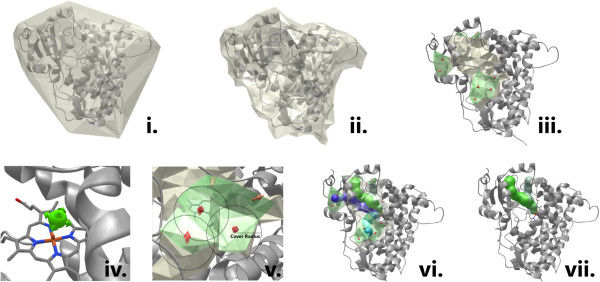
The computation of the tunnel is performed in several steps (see Figure 1) described in more detail in MOLE 2.0 publication:
- computation of the Delaunay triangulation/Voronoi diagram of the atomic centers,
- construction of the molecular surface, identification of cavities,
- identification of possible channel start points,
- identification of possible channel end points,
- localization of channels using ,
- filtering of the localized channels.
Calculation of channels
The channel computation is finished after the definition of starting and ending points for all of cavities, the Dijkstra’s Shortest Path Algorithm is used to find the channels between all pairs of starting and ending points (or the molecular surface if the algorithm reaches it before it finds the channel exit). The edge weight function used in the algorithm takes into account the distance to the surface of the closest vdW sphere and the edge length.
The channel centerline is represented as a 3D natural spline representation defined by the Voronoi diagram vertices that form the path found by the Dijkstra‘s algorithm.
The algorithm might find duplicate channels. Therefore, in the last post-processing step, the duplicate channels are removed according to Channel parameters.
Pore calculation
Pores are calculated differently than channels in the classical MOLE computation and is divided into two steps:
- finding of membrane region and
- calculation of the pore.
The pore computation starts with defining of the membrane region of the molecule. Firstly, MOLE is trying to find the structure on Orientations of Proteins in Membranes - OPM database (http://opm.phar.umich.edu/; Lomize,M.A., Lomize,A.L., Pogozheva,I.D. and Mosberg,H.I. (2006) OPM: Orientations of Proteins in Membranes Database. Bioinformatics, 22, 623–625).
If the structure cannot be found in the OPM database the MOLE continue in searching the membrane region by using the MEMEMBED program (Nugent,T. and Jones,D.T. (2013) Membrane protein orientation and refinement using a knowledge-based statistical potential. BMC Bioinformatics, 14, 276) which is able to predict the probable membrane region of the protein molecule.
When the membrane region definition is finished the pore end points are computed. The option Beta structure serves as the parameter for refinement of the membrane region prediction. The prediction of the membrane region highly depends on the secondary structure of the studied molecule.
Further reading
- Pravda L., Berka K., Sehnal D., Otyepka M., Svobodová Vařeková R., Koča J.Koča J, Svobodová Vařeková R, Pravda L, Berka K, Geidl S, Sehnal D, Otyepka M. Detection of Channels. Structural Bioinformatics Tools for Drug Design. 2016; Cham: Springer. 59–69.
- Simões T., Lopes D., Dias S., Fernandes F., Pereira J., Jorge J., Bajaj C., Gomes A. Geometric detection algorithms for cavities on protein surfaces in molecular graphics: a survey. Comput. Graph. Forum. 2017. Excellent review not only about different methods for channel analysis but also about the theory behind.
- Edelsbrunner, H., & Mücke, E. P. Three-dimensional alpha shapes. ACM Transactions on Graphics, 13(1), 43–72. 1994. Mathematical background of Voronoi diagrams construction used in MOLE algorithm.
Other Details
Origins
This option allows choosing of the start point by clicking to the ball which is pre-calculated inside the structure after upload of PDB code or your own structure from the file. After the click to the ball the selection will be created and this selection can be used as the start point. Similarly, the cavity may be also defined as the starting point but is necessary to first choose the cavity residues by clicking to the structure with CTRL+click and choose the specific amino acids localized in the cavity (Figure 2).
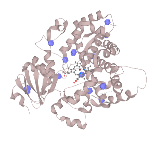
Another option is just selection of several residues by clicking to the structure and put this selection to the starting or ending point box (or other fields which can work with the selection of residues). In the same way, the sequence viewer can be also used for the selection of the starting point.
During the clicking to the individual residues the center of mass is calculated gradually and it is displayed as a clickable ball.
Visualization of results
Radius of channel/pore
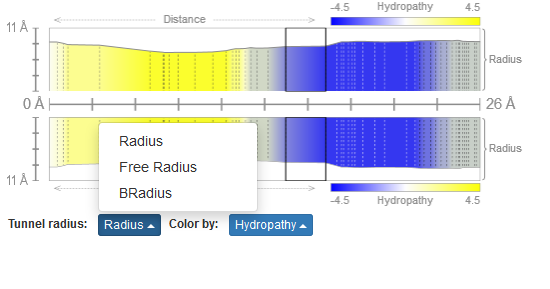
The MOLEonline offers three representations of the channel/pore radius (Figure 3):
- Radius – Radius of sphere within channel limited by three closest atoms
- Free Radius – Radius of sphere within channel limited by three closest main chain atoms in order to allow sidechain flexibility
- BRadius – Radius + RMSF calculated from B-factors of residues within individual layers

Calculation of physico-chemical properties
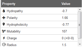
When the tunnel is computed the set of amino acids (side chains) lining the channel can be used for the physico-chemical properties computation (Figure 4). According to side chains composition, the set of physico-chemical properties is calculated (for lining amino acids side chains only):
Charge is calculated as a sum of charged amino acid residues (ARG, LYS, HIS = +1; ASP, GLU = -1)
Hydropathy is calculated as an average of hydropathy index assigned to residues according to the method of Kyte and Doolitle (Kyte, J. and Doolittle, R.F. (1982) A Simple Method for Displaying the Hydropathic Character of a Protein. J. Mol. Biol., 157, 105–132)
Hydropathy index is connected to hydrophilicity/hydrophobicity of amino acids (most hydrophilic is ARG = -4.5; most hydrophobic ILE = 4.5).
Hydrophobicity is calculated as an average of normalized hydrophobicity scales by Cid et al. (Cid, H., Bunster, M., Canales, M. and Gazitúa, F. (1992) Hydrophobicity and structural classes in proteins. Protein Eng. Des. Sel., 5, 373–375).
Most hydrophilic amino acid according to hydrophobicity value is GLU (-1.140) and the most hydrophobic is ILE (1.810).
Polarity is calculated as an average of amino acid polarities assigned according to the method of Zimmerman et al. (Zimmerman, J.M., Eliezer, N. and Simha, R. (1968) The Characterization of Amino Acid Sequences in Proteins by Statistical Methods. J. Theor. Biol., 21, 170–201).
Polarity ranges from completely nonpolar amino acids (ALA, GLY = 0.00) through polar residues (e.g. SER = 1.67) towards charged residues (GLU = 49.90, ARG = 52.00).
Lipophilicity (logP-scale) is calculated as octanol/water partition coefficients of Cβ fragments of side-chains and mainchain (-0.86) via www.chemicalize.org.
LogP values ranges from lipophobic fragments (ASN -1.03; SER -0.52; GLN -0.33; THR -0.16) through acids (ASP -0.22; GLU 0.48) and bases (ARG -0.08; HIS -0.01; LYS 0.7), to sulphur-containing (CYS 0.84; MET 1.48), aliphatic (ALA 1.08; VAL 1.8; PRO 1.8; LEU 2.08; ILE 2.24) to most lipophilic aromatic residues (TYR 2.18; PHE 2.49; TRP 2.59). GLY has no sidechain fragment and therefore its value is set to 0.
Lipophilicity (logD-scale) is calculated as octanol/water distribution coefficients of Cβ fragments of side-chains and mainchain (-0.86) at pH 7.4 via www.chemicalize.org. Distribution coefficient take into account ionization of compounds.
LogD values ranges from highly lipophobic charged fragments (ASP -3.00; ARG -2.49; GLU -2.12; LYS -1.91) through polar ones (ASN -1.03; SER -0.52; GLN -0.33; THR -0.16, HIS -0.11) to sulphur-containing (CYS 0.84; MET 1.48), aliphatic (ALA 1.08; VAL 1.8; PRO 1.8; LEU 2.08; ILE 2.24) to most lipophilic aromatic residues (TYR 2.18; PHE 2.49; TRP 2.59). GLY has no sidechain fragment and therefore its value is set to 0.
Solubility (logS-scale) is calculated as water solubility of Cβ fragments of side-chains and mainchain (0.81) at pH 7.4 via www.chemicalize.org. Our estimated logS value is a unit stripped logarithm (base 10) of the solubility measured in mol/liter and it is a measure how well can be individual residues interacting with water molecules.
LogS values ranges from lowest solubility of aromatic residues (TRP -2.48: PHE -1.81; TYR -1.44;) followed by aliphatic (LEU -1.79; ILE -1.85; PRO -1.3; VAL -1.3; ALA 0.59) and sulphur-containing residues (MET -0.72; CYS 0.16) up to polar ones (HIS -0.2; GLN 0.13; ASN 0.54; THR 0.77; SER 1.11) whereas the most water molecules will attract charged residues (LYS 1.46; ARG 1.63; GLU 2.23; ASP 2.63). GLY has no sidechain fragment and therefore its value is set to 0.
Mutability is calculated as an average of relative mutability index (Jones,D.T., Taylor,W.R. and Thornton,J.M. (1992) The Rapid Generation of Mutation Data Matrices from Protein Sequences. Bioinformatics, 8, 275–282). Relative mutability is based on empirical substitution matrices between similar protein sequences.
It is high wherever amino acid can be easily substituted for another e.g. in case of small polar amino acids (SER = 117, THR = 107, ASN = 104) or in case of small aliphatic amino acids (ALA = 100, VAL = 98, ILE = 103). On the other hand it is low when amino acid plays important structural role such as in case of aromatic amino acids (TRP = 25, PHE = 51, TYR = 50) or in case of special amino acids (CYS = 44, PRO = 58, GLY = 50). Specific example of amino acid with low relative mutability is the most abundant amino acid /LEU = 54) which has the highest probability to mutate back to itself.
Ionizable residues can be also viewed in the channel profile or directly as selection on the visualized structure.
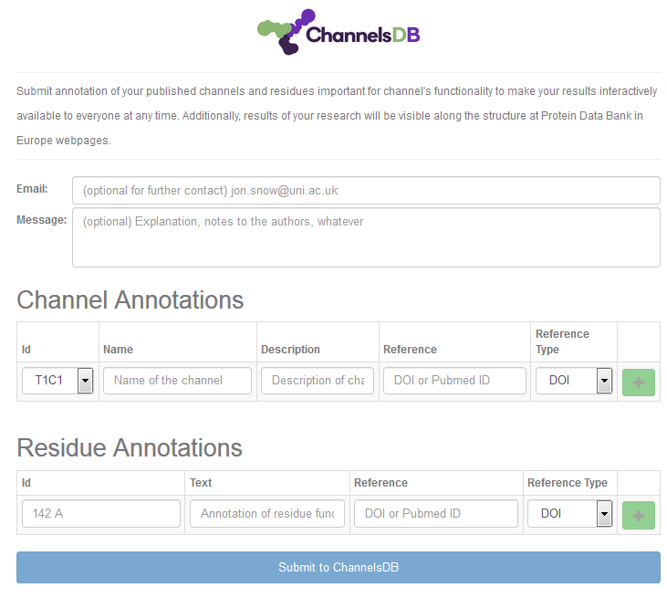
Annotations
You can contribute to the ChannelsDB database (http://ncbr.muni.cz/ChannelsDB/) by Annotation button in the upper left corner of the visualization window. Annotation can be easily written to the boxes in the Annotation window and channels selected from those calculated within the window (Figure 5).